I’m currently working on the Python code to control a simulated version of my latest bipedal robot design in PyBullet. My focus over the past few weeks was getting the operational space control to work (many thanks to Travis DeWolf’s incredibly helpful blog). After finally getting it to work properly, I have decided to share my math in the hopes of providing a useful example for anyone else having trouble with this. There really aren’t enough resources on the internet that explain this in a succinct manner.
Solving for the transformation matrices and centers of motion correctly is the trickiest part of the process, and deceptively so. For more information on how to set up the transformation matrices, I recommend this Youtube tutorial and this blog post.
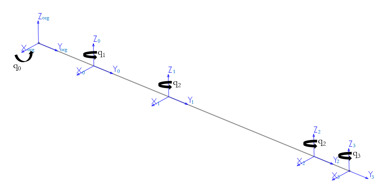
I find it easiest to solve for the transformation matrices by “stringing” the robot out, as shown below, such that all of the joints’ coordinate systems are oriented the same way. This saves you from having to perform additional linear algebra operations, which would raise your chances of making a mistake.
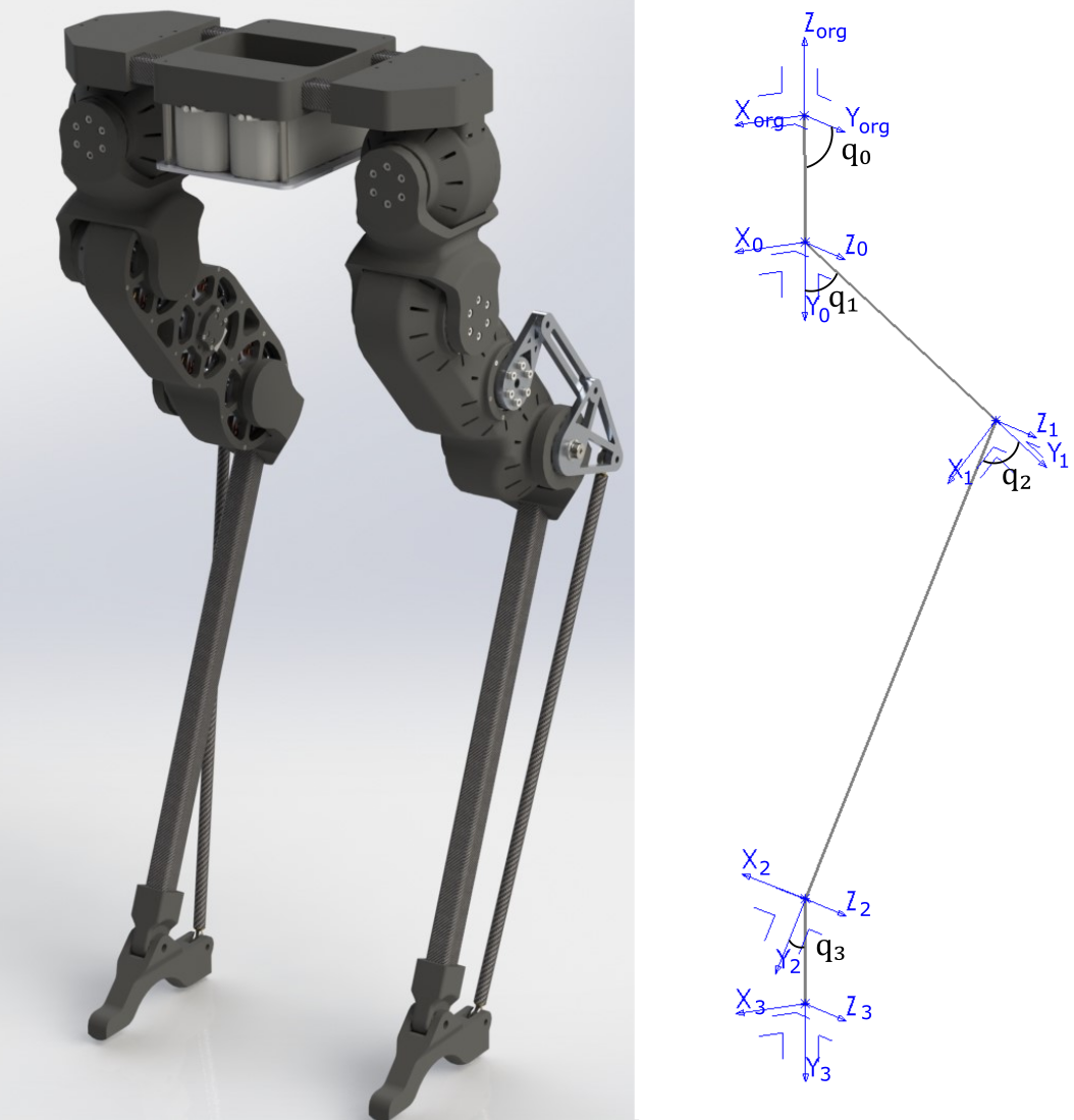
Shown below are the transformation matrices. The first transformation represents an x-axis rotation. See the first joint in the kinematic diagram above for reference. Transformations (2) through (4) are z-axis rotations. Despite the z-axis pointing up in the world coordinate system, the default angle (90 degrees) for the first x-axis rotation points the z-axis of the second through fourth joints parallel to the y-axis of the WCS.
$$ \begin{equation} {}_{org}^0 T = \begin{bmatrix} 1 & 0 & 0 & 0 \newline 0 & \cos{(q_{0})} & - \sin{(q_{0})} & L_{0}\cos{(q_{0})} \newline 0 & \sin{(q_{0})} & \cos{(q_{0})} & L_{0}\sin{(q_{0})} \newline 0 & 0 & 0 & 1 \end{bmatrix} \end{equation} $$ $$ \begin{equation} {}_0^1 T = \begin{bmatrix} \cos{(q_{1} )} & - \sin{(q_{1} )} & 0 & -L_{1} \sin{(q_{1} )} \newline \sin{(q_{1} )} & \cos{(q_{1} )} & 0 & L_{1} \cos{(q_{1} )} \newline 0 & 0 & 1 & 0 \newline 0 & 0 & 0 & 1 \end{bmatrix} \end{equation} $$ $$ \begin{equation} {}_1^2 T = \begin{bmatrix} \cos{(q_{2} )} & - \sin{(q_{2} )} & 0 & -L_{2} \sin{(q_{2} )} \newline \sin{(q_{2} )} & \cos{(q_{2} )} & 0 & L_{2} \cos{(q_{2} )} \newline 0 & 0 & 1 & 0 \newline 0 & 0 & 0 & 1 \end{bmatrix} \end{equation} $$ $$ \begin{equation} {}_2^3 T = \begin{bmatrix} \cos{(q_{3} )} & - \sin{(q_{3} )} & 0 & -L_{3} \sin{(q_{3} )} \newline \sin{(q_{3} )} & \cos{(q_{3} )} & 0 & L_{3} \cos{(q_{3} )} \newline 0 & 0 & 1 & 0 \newline 0 & 0 & 0 & 1 \end{bmatrix} \end{equation} $$Next, the locations for the centers of mass at each link are found, where $l_0$, $l_1$, $l_2$, and $l_3$ represent the distance of the center of mass from the base joint of each link, along a line connecting the base joint to the next joint. Keep in mind that the centers of mass may not be located directly along a line from one joint to the next in any given robot link, and that in this case I am able to make this approximation for the purpose of mathematical simplicity.
$$ \begin{equation} com_0 = \begin{bmatrix} 0 \newline l_{0} \cos{(q_{0} )} \newline l_{0} \sin{(q_{0} )} \newline 1 \end{bmatrix} \end{equation} $$
$$ \begin{equation} com_1 = \begin{bmatrix} {-l_{1} \sin{(q_{1} )}} \newline l_{1} \cos{(q_{1} )} \newline 0 \newline 1 \end{bmatrix} \end{equation} $$
$$ \begin{equation} com_2 = \begin{bmatrix} -l_{2} \sin{(q_{2} )} \newline l_{2} \cos{(q_{2} )} \newline 0 \newline 1 \end{bmatrix} \end{equation} $$
$$ \begin{equation} com_3 = \begin{bmatrix} -l_{3} \sin{(q_{3} )} \newline l_{3} \cos{(q_{3} )} \newline 0 \newline 1 \end{bmatrix} \end{equation} $$
The end-effector offset (Equation 9) should also be kept in mind, but in my case I don’t need an offset from the end-effector. As such, I’m expressing it as zero.
$$ \begin{equation} x_{ee} = \begin{bmatrix} 0 \newline 0 \newline 0 \newline 1 \end{bmatrix} \end{equation} $$
Next, I solved for the full transformation matrices from the origin to each joint. This isn’t necessary for the first joint, because it’s already in the base coordinate system.
$$ \begin{equation} _{org}^1 T = _{org}^0 T _0^1 T \end{equation} $$
$$ \begin{equation} _{org}^2 T = _{org}^0 T _0^1 T _1^2 T \end{equation} $$
$$ \begin{equation} _{org}^3 T = _{org}^0 T _0^1 T _1^2 T _2^3 T \end{equation} $$
Now, the Jacobian for each COM and the end-effector can be found as a matrix of its partial derivatives with respect to each joint qᵢ. Both linear and angular velocities must be accounted for, so I have $x$, $y$, $z$, $\omega_x$, $\omega_y$, $\omega_z$ to deal with.
$$ \begin{equation} Jacobian = \begin{bmatrix} \frac{\partial x}{\partial q_0} & \frac{\partial x}{\partial q_1} & \frac{\partial x}{\partial q_2} & \frac{\partial x}{\partial q_3} \newline \frac{\partial y}{\partial q_0} & \frac{\partial y}{\partial q_1} & \frac{\partial y}{\partial q_2} & \frac{\partial y}{\partial q_3} \newline \frac{\partial z}{\partial q_0} & \frac{\partial z}{\partial q_1} & \frac{\partial z}{\partial q_2} & \frac{\partial z}{\partial q_3} \newline \frac{\partial \omega_x}{\partial q_0} & \frac{\partial \omega_x}{\partial q_1} & \frac{\partial \omega_x}{\partial q_2} & \frac{\partial \omega_x}{\partial q_3} \newline \frac{\partial \omega_y}{\partial q_0} & \frac{\partial \omega_y}{\partial q_1} & \frac{\partial \omega_y}{\partial q_2} & \frac{\partial \omega_y}{\partial q_3} \newline \frac{\partial \omega_z}{\partial q_0} & \frac{\partial \omega_z}{\partial q_1} & \frac{\partial \omega_z}{\partial q_2} & \frac{\partial \omega_z}{\partial q_3} \newline \end{bmatrix} \end{equation} $$So far I haven’t explained angular velocity. This I have solved separately, and it’s quite simple as long as your robot is serial and doesn’t have spherical joints. The partial derivative for the angular velocity w.r.t. each joint is expressed as 1 if that joint rotates along that axis, and 0 if it doesn’t. For example, in $J_0$ (Equation 14), joint $q_0$ rotates around the x axis, so the partial derivative of $\omega_x$ w.r.t. $q_0$ is 1. In $J_1$ (Equation 15), joint $q_1$ rotates about the z axis, so the partial derivative of $\omega_z$ w.r.t. $q_1$ is 1.
$$ \begin{equation} J_0 = Jacobian(com_0) = \begin{bmatrix} 0 & 0 & 0 & 0 \newline - l_{0} \sin{(q_{0} )} & 0 & 0 & 0 \newline l_{0} \cos{(q_{0} )} & 0 & 0 & 0 \newline 1 & 0 & 0 & 0 \newline 0 & 0 & 0 & 0 \newline 0 & 0 & 0 & 0 \end{bmatrix} \end{equation} $$I can only show the first two Jacobians here, as the rest are too long to fit on the screen. You’ll notice that the Jacobians for the centers of motion of each link ($J_0$, $J_1$, $J_2$, and $J_3$) are calculated as a function of the transformation matrix from the link’s base joint to the origin multiplied by that link’s center of motion. This confused me the first time around, and I don’t want you, the reader, to make the same mistake.
For example, in the case of $J_1$ (the Jacobian for the second link), the transformation matrix from joint 0 to the world coordinate frame (origin) is multiplied by $com_1$, the center of motion of the link between joints 0 and 1 (the first and second joints, so the second link).
For $J_0$ (the Jacobian for the first link), no transformation matrix is required because the first joint ($q_0$) is already in the base coordinate system.
I’m probably just confusing you more because my joint indexing starts at zero, but that’s for programming purposes and is standard…
$$ J_1 = Jacobian(_{org}^0 T com_1) = $$
$$ \begin{equation} \begin{bmatrix} 0 & - l_{1} \cos{(q_{1} )} & 0 & 0 \newline - (L_{0} + l_{1} \cos{(q_{1} )}) \sin{(q_{0} )} & - l_{1} \sin{(q_{1} )} \cos{(q_{0} )} & 0 & 0 \newline (L_{0} + l_{1} \cos{(q_{1} )}) \cos{(q_{0} )} & - l_{1} \sin{(q_{0} )} \sin{(q_{1} )} & 0 & 0 \newline 1 & 0 & 0 & 0 \newline 0 & 0 & 0 & 0 \newline 0 & 1 & 0 & 0 \end{bmatrix} \end{equation} $$
$$ \begin{equation} J_2 = Jacobian(_{org}^1 T com_2) \end{equation} $$
$$ \begin{equation} J_3 = Jacobian(_{org}^2 T com_3) \end{equation} $$
$$ \begin{equation} J_{EE} = Jacobian(_{org}^3 T x_{ee}) \end{equation} $$So there you have it. After several headaches, I was able to verify that this setup works in simulation. The chief cause of my problems was that I had solved for the transformation matrices incorrectly! Everything else is easy–though it looks intimidating, all of the symbolic math can be computationally solved by Matlab/Octave. Just remember…
$$ \begin{equation} \text{garbage}_{in} = \text{garbage}_{out} \end{equation} $$Last edited 2026-06-02.