Intro to Robot Simulation, Part 1: Point Masses

So, you want to write your own dynamic robot simulation from scratch.

Let’s start with one of the simplest possible dynamical systems: a vertically constrained point mass. Think of it as a rocket locked to a linear rail.

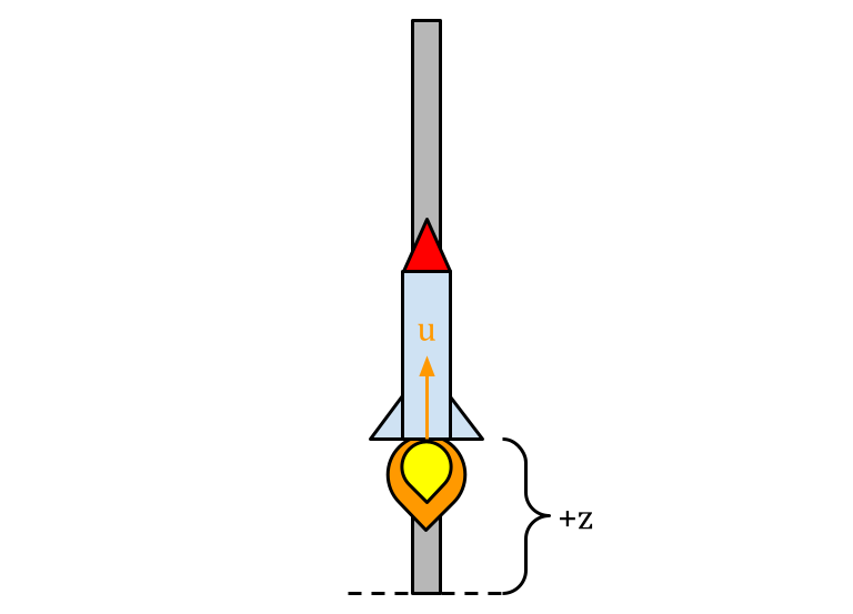
The rocket cannot rotate or translate laterally; it can only move up or down, and can it only control this by either exerting an upward force or letting gravity take its course.

Therefore, we can solve for the acceleration of the rocket as follows:

$$ \begin{equation} \ddot{z} = \frac{u}{m} - 9.81 \end{equation} $$

Where $\ddot{z}$ is the rocket’s vertical acceleration, $u$ is the force exerted by the rocket, $m$ is the rocket’s mass, and the additional term is gravity.

Writing a CT State Space Model

We begin by rewriting Eq(1) as a continuous-time (CT) linear state space representation of the system. Our state vector, usually denoted by $X$, is composed of the vertical position $z$ and its vertical velocity $\dot{z}$.

The purpose of the CT state-space representation is to solve for the derivative of $X$:

For the rocket-on-a-rail, this can be solved as such:

Note the $A$ matrix (AKA “the state matrix”), which governs how $X$ affects $\dot{X}$. In this case, the only relation is that $\dot{z} = \dot{z}$.

Secondly, the B matrix (AKA “the input matrix”) governs how the control input $U$ affects $\dot{X}.$

Finally, the G matrix represents a disturbance, which in this case is the constant acceleration acting on the system due to gravity.

From Continuous-Time to Discrete-Time

Continuous-time state space models represent the dynamics of a system with respect to time. Let’s focus on the linear time-invariant (LTI) case to keep things simple (This means that the A and B matrices are not functions of time, e.g. $A(t)$).

$$ \begin{equation} \dot{X}(t) = A X(t) + B U(t) \end{equation} $$

Now imagine if we wanted to simulate such a system. We would need to measure the state $X(t)$ for various values of $t$. This would not be possible, as we are only solving for its derivative, $\dot{X}(t)$!

Luckily, there is a solution for the LTI case that makes this possible:

$$ \begin{equation} X(t) = e^{(t - t_0)A} X(t_0) + \int^t_{t_0} e^{A (t-\tau)} B u(\tau) d\tau \end{equation} $$

The problem, of course, is that it requires the calculation of a matrix exponential, $e^A$, the solution for which is an infinite series.

The main takeaway here is that any attempt to simulate a LTI state space system can be interpreted as an approximation of the matrix exponential. There are many ways to do this (at least nineteen!), but I will only cover a few here.

Okay, anyway, we can solve for $X(t)$ now. But do we want to find $X$ for any arbitrary $t$? Actually, it is most convenient to “step” through time at a constant rate. The time between each step is known as a timestep and will be written as $dt$ here.

With this in mind, we should now be concerned with discrete timesteps $k$, and as such we rewrite the model in discretized form as follows: $$ \begin{equation} X_{k+1} = A_d X_k + B_d U_k + G_d \end{equation} $$

Note that instead of calculating $\dot{X}$, we are now attempting to calculate $X_{k+1}$, which is just $X$ at the next timestep.

The expm() Method

The most obvious way to solve for the state at each timestep is to simply call a function that solves the matrix exponential. In this case, we use scipy.linalg.expm(). This also happens to be one the most accurate methods (although it’s still technically an approximation), and one of the most computationally expensive.

The code in this guide is written in Python. We will start by importing necessary libraries and defining the constants.

import numpy as np
from scipy.linalg import expm
import matplotlib.pyplot as plt

n_x = 2  # length of state vector
n_u = 1  # length of control vector
m = 10  # mass of the rocket in kg
A = np.array([[0, 1],
              [0, 0]])
B = np.array([[0],
              [1/m]])
G = np.array([[0], [-9.81]])
dt = 0.001  # timestep size

Next, we write a function to calculate the discretized dynamics using expm(). Because expm() only accepts square matrices, and $B$ and $G$ are not square, we perform a little trick here where we merge $A$, $B$, and $G$ into one big square matrix using a few extra rows of zeros. Then we extract the discretized $A_d$, $B_d$, and $G_d$ from the result.

def dynamics_dt(X, U):
    ABG = np.vstack((np.hstack((A, B, G)), np.zeros((n_u + 1, n_x + n_u + 1))))
    M = expm(ABG * dt)
    Ad = M[0:n_x, 0:n_x]
    Bd = M[0:n_x, n_x:n_x + n_u]
    Gd = M[0:n_x, n_x + n_u:]   
    X_next = Ad @ X + Bd @ U + Gd.flatten()
    return X_next

Now we can set the simulation up, run it, and plot the result.

N = 1000  # number of timesteps
X_hist = np.zeros((N, n_x))  # array of state vectors for each timestep
X_hist[0, :] = np.array([[1, 0]])
U_hist = np.zeros((N-1, n_u)) # array of control vectors for each timestep

for k in range(N-1):
    X_hist[k+1, :] = dynamics_dt(X_hist[k, :], U_hist[k, :])

plt.plot(range(N), X_hist[:, 0], label='expm')
plt.title('Body Position vs Time')
plt.ylabel("z (m)")
plt.xlabel("timesteps")
plt.show()

The full code can be found here. You should get the following result:

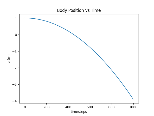
As you can see, the point mass accelerates downward due to gravity. Simple stuff.

The Euler Method

There is a broad class of methods known as Runge-Kutta, which can be used to discretize any transient problem, including nonlinear ones. The Euler method is probably the simplest of those, which is why I am covering it here. Unlike the previous discretization method, it is extremely computationally efficient, albeit inaccurate and unstable. The Euler method is the standard discretization method used in video games, where physical accuracy is considered “optional”.

Like I said, the Euler method is simple. It assumes that the state at the next timestep is simply the current state plus the state derivative multiplied by the timestep size. This makes a lot of intuitive sense.

$$ \begin{equation} X_{k+1} = X_k + \dot{X_k}\text{dt} \end{equation} $$

Let’s see how this looks in code:

def dynamics_ct(X, U):
    dX = A @ X + B @ U + G.flatten()
    return dX

def integrator_euler(dyn_ct, xk, uk):
    X_next = xk + dt * dyn_ct(xk, uk)
    return X_next

Now, replace the for loop from earlier with the following:

for k in range(N-1):
    X_hist[k+1, :] = integrator_euler(dynamics_ct, X_hist[k, :], U_hist[k, :])

Your resulting plot should look exactly the same.

The Fourth-Order Runge-Kutta Method

Despite its computational efficiency, the Euler method is not ideal for robotics. Higher-order Runge-Kutta methods are generally preferred due to their superior accuracy and stability. The fourth-order Runge-Kutta method (RK4) is one of the most popular.

For brevity, I won’t explain how/why it works here, but you can try it out by replacing the integrator_euler() function with the following:

def integrator_rk4(dyn_ct, xk, uk):
    f1 = dyn_ct(xk, uk)
    f2 = dyn_ct(xk + 0.5 * dt * f1, uk)
    f3 = dyn_ct(xk + 0.5 * dt * f2, uk)
    f4 = dyn_ct(xk + dt * f3, uk)
    return xk + (dt / 6.0) * (f1 + 2 * f2 + 2 * f3 + f4)

For such a simple setup, you won’t notice much of a difference between these methods until you turn the timestep size way up. The following plot compares all three methods covered here using a timestep size of a tenth of a second.

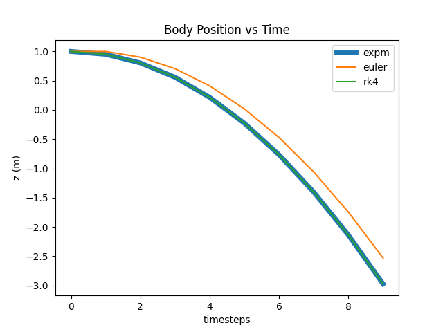
The expm result should be taken as “ground truth”. As you can see, the Euler method visibly diverges from “truth”, but it is still not possible to distinguish the RK4 results from expm.

Adding Control

One more thing. After the first half a second, let’s add a 1000N force to the control vector applied over the course of a quarter second and see what happens.

N = 5000  # number of timesteps
X_hist = np.zeros((N, n_x))  # array of state vectors for each timestep
X_hist[0, :] = np.array([[1, 0]])
U_hist = np.zeros((N-1, n_u)) # array of control vectors for each timestep

U_hist[500:750, :] = 1000  # HERE!

for k in range(N-1):
    X_hist[k+1, :] = dynamics_dt(X_hist[k, :], U_hist[k, :])

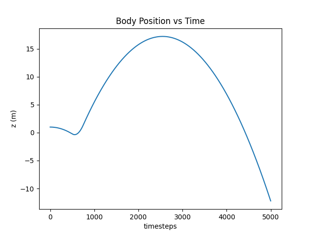
Whee!

Next Steps

In the next part of this series, I will cover how contact is simulated, so that the point mass can bounce off the ground.