Okay, so we can simulate a floating point mass subject to arbitrary forces. Let’s now think about what happens when our point mass hits the ground.
Assuming 100% stiff, inelastic impact, we would get the following position, velocity, and acceleration trajectories:
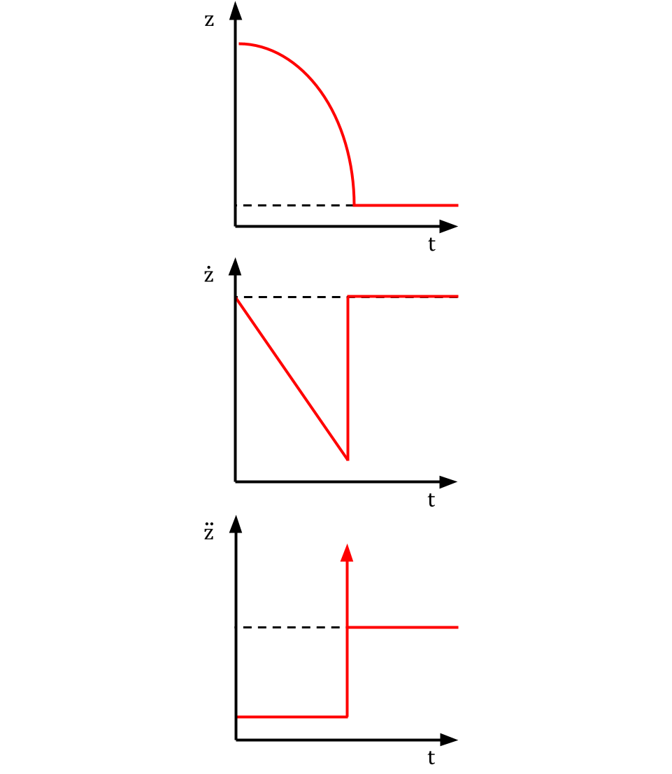
Notably, the acceleration at impact approaches infinity, which would be very difficult to simulate–it would require infinitesimal timesteps. Of course, in reality there is no such thing as a perfectly stiff and inelastic collision, but in the field of robotics we are often concerned with relatively stiff collisions which cause decelerations on the order of microseconds.
So how do we do that?
Generalizing grossly, there are three overarching categories of methods for simulating contact, which I will cover here.
The Hybrid Method
In this method, a “guard function” explicitly checks for contact on every timestep. If it is triggered, a “jump map” function is called, which applies impact discontinuities. Additionally, separate dynamics models can be used depending on whether or not the object is currently in contact.
Let’s look at a code example. We will use the same state-space system from Part 1, a vertically constrained point mass.
import numpy as np
import plotting

n_x = 2  # length of state vector
n_u = 1  # length of control vector
m = 10  # mass of the rocket in kg
A = np.array([[0, 1], [0, 0]])
B = np.array([[0], [1 / m]])
G = np.array([[0], [-9.81]])
dt = 0.001  # timestep size


def dynamics_ct(X, U):
    dX = A @ X + B @ U + G.flatten()
    return dX


def integrator_euler(dyn_ct, xk, uk):
    X_next = xk + dt * dyn_ct(xk, uk)
    return X_next
Next, we define our “jump map”. This function will be called whenever the object passes through the ground. It rewrites the position to avoid interpenetration. In addition, it rewrites the velocity based on a chosen coefficient of restitution $e$ and calculates the ground reaction force necessary for this to occur. Here we have set $e$ to 0.7 arbitrarily.
e = 0.7  # coefficient of restitution
def jump_map(X):  #
    X[0] = 0  # reset z position to zero
    v_before = X[1]  # velocity before impact
    v_after = (
        -e * v_before
    )  # reverse velocity and multiply by coefficient of restitution
    a = (v_after - v_before) / dt  # acceleration
    F = m * a  # get ground reaction force
    X[1] = v_after  # velocity after impact
    return X, F
Finally, we iterate through the timesteps. The jump map is called whenever the object’s position value is negative.
N = 1000  # number of timesteps
X_hist = np.zeros((N, n_x))  # array of state vectors for each timestep
F_hist = np.zeros((N, 1))  # array of state vectors for each timestep
X_hist[0, :] = np.array([[1, 0]])  # start from a height of 1 m
U_hist = np.zeros((N - 1, n_u))  # array of control vectors for each timestep

for k in range(N - 1):
    if X_hist[k, 0] <= 0:  # guard function
        X_hist[k, :], F_hist[k, :] = jump_map(
            X_hist[k, :]
        )  # dynamics rewrite based on impact
    X_hist[k + 1, :] = integrator_euler(dynamics_ct, X_hist[k, :], U_hist[k, :])
Click here for the full code.
Let’s look at the results:

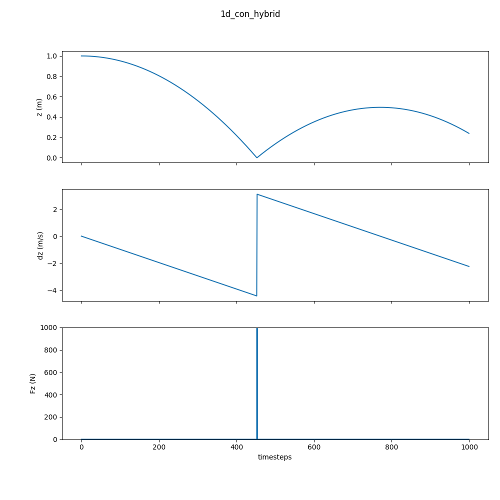
Everything here seems reasonable, except that the ball is probably unrealistically stiff for how bouncy it is.
Also, set $e = 0$ to see what an inelastic collision looks like:
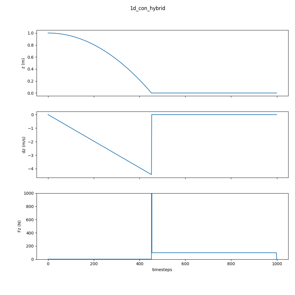
Neat!
Smooth Contact
In this method, contact is approximated as a spring-damper system. The trick here is that the spring-damper model is used at all times, regardless of whether or not contact should be occurring.
Let’s look at the code.
The function below takes as inputs the distance of the object from the ground and its speed. It then calculates the ground reaction force based on user-tuned spring and damping constants.
def get_grf(X: np.ndarray) -> float:
    z = X[0]
    dz = X[1]
    k = 0.01  # spring constant
    b = 0.1  # damping constant
    amp = 1500  # desired max force
    c = amp * 0.5 / k
    distance_fn = -c * np.tanh(z * 100) + c
    F_spring = k * distance_fn
    F_damper = -b * dz * distance_fn
    grf = F_spring + F_damper
    return grf
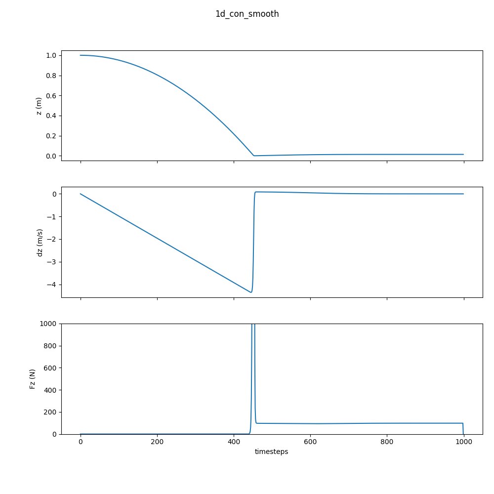
If we plot this function, we see that the force drops off precipitously as distance from the ground increases.
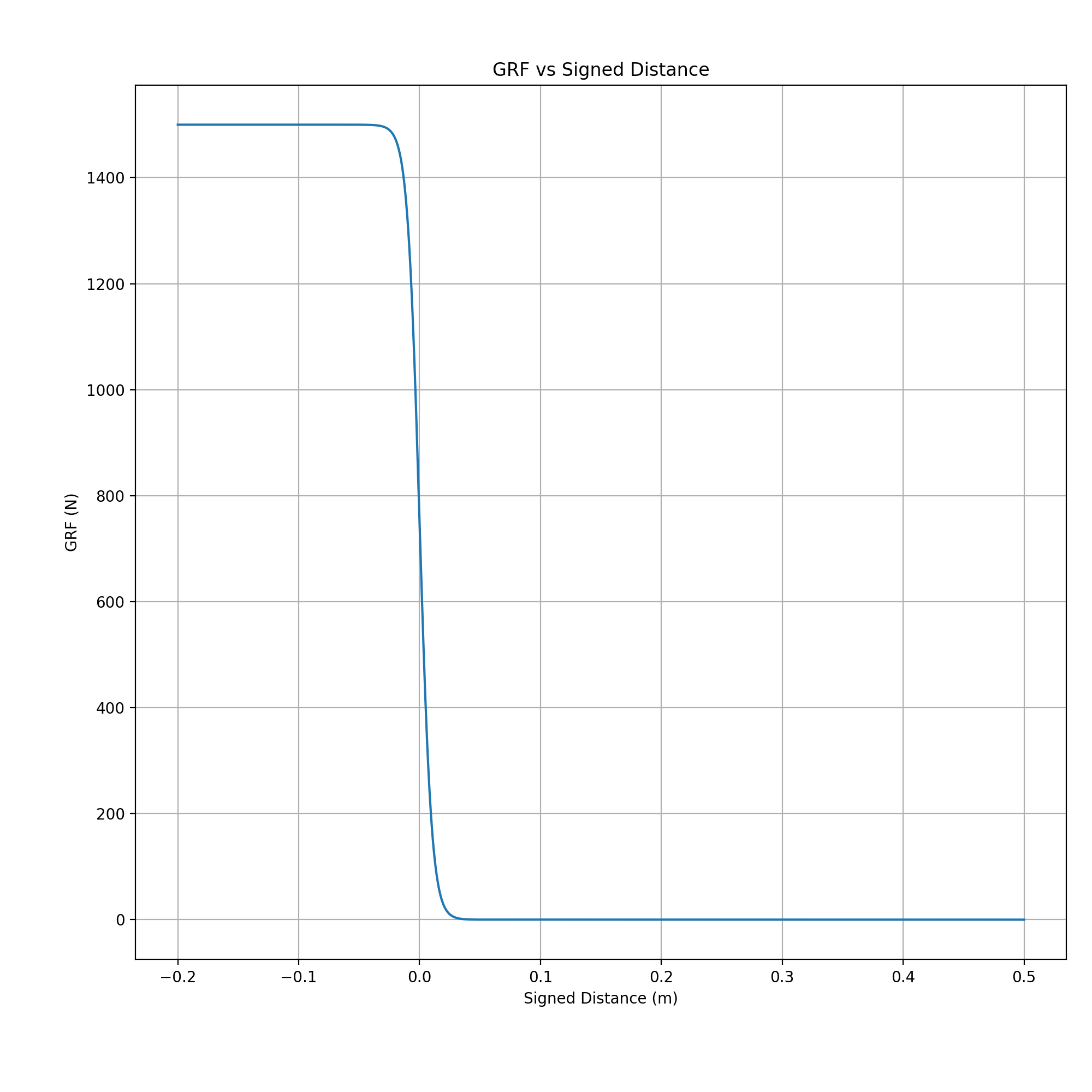
I chose a $\tanh$ relationship between input and output somewhat arbitrarily to achieve this effect. As a consequence there is a max ground reaction force possible, which isn’t great. But you can tune it.
Let’s look at the rest of the code now. The dynamics and integrator are exactly the same as in the hybrid example.
But the simulation is simpler. There’s no explicit check for interpenetration; the spring-damper function is simply called on every timestep. When the object isn’t close to the ground, the forces are just too small to notice. This is what makes the smooth contact method both beautifully elegant, and just wrong.
n_x = 2  # length of state vector
n_u = 1  # length of control vector
m = 10  # mass of the rocket in kg
A = np.array([[0, 1], [0, 0]])
B = np.array([[0], [1 / m]])
G = np.array([[0], [-9.81]])
dt = 0.001  # timestep size

def dynamics_ct(X, U):
    dX = A @ X + B @ U + G.flatten()
    return dX

def integrator_euler(dyn_ct, xk, uk):
    X_next = xk + dt * dyn_ct(xk, uk)
    return X_next

N = 1000  # number of timesteps
X_hist = np.zeros((N, n_x))  # array of state vectors for each timestep
F_hist = np.zeros((N, n_u))  # array of state vectors for each timestep
X_hist[0, :] = np.array([[1, 0]])

for k in range(N - 1):
    F_hist[k, :] = get_grf(X_hist[k, :])  # get spring-damper force
    X_hist[k + 1, :] = integrator_euler(dynamics_ct, X_hist[k, :], F_hist[k, :])
Click here for the full code.
Note that I’m feeding the ground reaction force in to where the control vector is supposed to go. Since both the control and GRF can apply a vertical force, this is a little cheat to let me write less lines of code.
Let’s look at the results. Pretty good!

Time-Stepping
In this method, an optimization problem is solved on each timestep to compute the contact forces required to satisfy interpenetration constraints.
Ideally, the system is described by the following four constraints. The first is our discrete-time system dynamics. Here, $X_k$ and $U_k$ are inputs and we want to solve for $X_{k+1}$ and $f_k$, where $f_k$ represents the reaction force between the ground and the point mass. Out of a convenient contrivance, $f_k$ uses the same input matrix $B_d$ as the control input $U_k$.
$$ \begin{equation} X_{k+1} = A_dX_k + B_dU_k + B_df_k + G_d \end{equation} $$
Secondly, we have our interpenetration constraint. This just says that the point mass must stay above the ground. As a reminder, $z_{k+1}$ is an element of $X_{k+1}$. $$ \begin{equation} z_{k+1} \geq 0 \end{equation} $$
Thirdly, we constrain the ground reaction force to be positive only. If it were negative, the ground would be pulling on the mass.
$$ \begin{equation} f_k \geq 0 \end{equation} $$
And finally, we have what is known as the complementarity constraint. This is a pretty neat trick. In order for the constraint to be satisfied, either $f_k$ or $z_{k+1}$ must be equal to zero at any given timestep. Therefore, when the object is not touching the ground, $f_k$ must be zero.
$$ \begin{equation} f_k z_{k+1} = 0 \end{equation} $$
The Optimization Problem
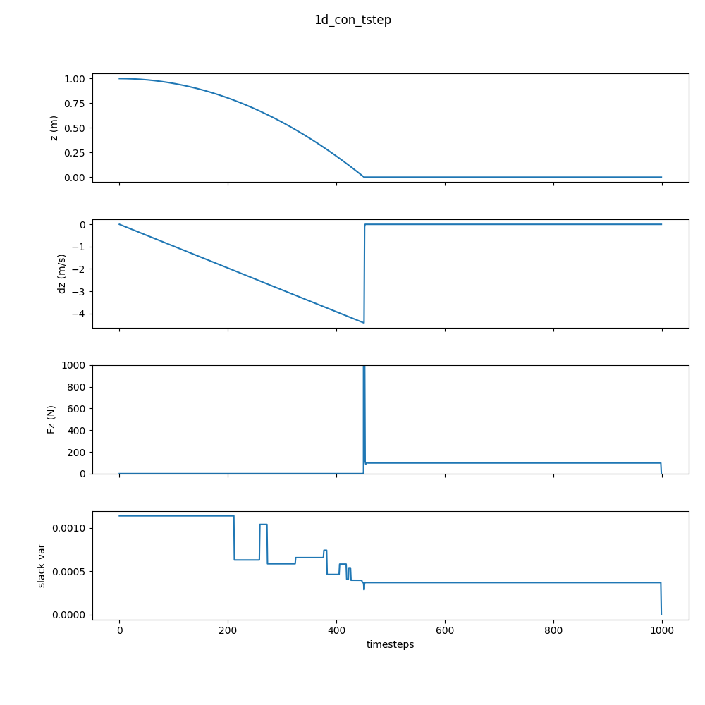
To practically implement this in an easy and accessible way, we will be using the IPOPT solver, which is broadly available. Bear in mind that you really need to write a custom solver to do this properly. But to make this solvable with IPOPT, we have to add a slack variable, denoted by $s$, to “relax” the discrete switching behavior of the complementarity constraint.
The optimization problem is as shown below. We attempt to minimize $s^2$ in the objective function, as opposed to just $s$, because it penalizes larger values more severely.
$$ \begin{align} \min_{X_{k+1}, f_k, s_k} \quad & s_k^2 \\ \textrm{s.t.} \quad & A_dX_k + B_dU_k + B_df_k + G_d - X_{k+1} = 0 \\ & s_k - f_k z_{k+1} \geq 0 \\ & z_{k+1} \geq 0 \\ & f_k \geq 0 \\ & s_k \geq 0 \\ \end{align} $$The Code
Starting with standard setup stuff, except that we are going to use the semi-implicit Euler method, which performs better here than other integrators. The only difference between it and the regular Euler method is that it uses the velocity term from the next ($k+1$) timestep.
import numpy as np
import plotting
import casadi as cs

n_a = 2  # length of state vector
n_u = 1  # length of control vector
m = 10  # mass of the particle in kg
g = 9.81  # gravitational constant
A = np.array([[0, 1], [0, 0]])
B = np.array([[0], [1 / m]])
G = np.array([[0], [-g]])
dt = 0.001  # timestep size

def dynamics_ct(X, U):
    dX = A @ X + B @ U + G.flatten()
    return dX


def integrator_euler_semi_implicit(dyn_ct, xk, uk, xk1):
    xk_semi = cs.SX.zeros(n_a)
    xk_semi[0] = xk[0]
    xk_semi[1] = xk1[1]
    X_next = xk + dt * dyn_ct(xk_semi, uk)
    return X_next

X_0 = np.array([1, 0])
N = 1000
X_hist = np.zeros((N, n_a))  # array of state vectors for each timestep
F_hist = np.zeros(N)  # array of z GRF forces for each timestep
s_hist = np.zeros(N)  # array of slack var values for each timestep
X_hist[0, :] = X_0
U_hist = np.zeros((N - 1, n_u))  # array of control vectors for each timestep
Here is where we define the optimization problem. We are using CaSaDi, a library for numerical optimization that has IPOPT built-in.
# initialize casadi variables
Xk1 = cs.SX.sym("Xk1", n_a)  # X(k+1), state at next timestep
F = cs.SX.sym("F", n_u)  # force
s = cs.SX.sym("s", 1)  # slack variable
X = cs.SX.sym("X", n_a)  # state
U = cs.SX.sym("U", n_u)  # controls

zk1 = Xk1[0]  # vert pos
dzk1 = Xk1[1]  # vertical vel

obj = s**2

constr = []  # init constraints
# dynamics
constr = cs.vertcat(
    constr, cs.SX(integrator_euler_semi_implicit(dynamics_ct, X, U + F, Xk1) - Xk1)
)
# relaxed complementarity
constr = cs.vertcat(constr, cs.SX(s - F * zk1))

opt_variables = cs.vertcat(Xk1, F, s)
# parameters = X
parameters = cs.vertcat(X, U)
lcp = {"x": opt_variables, "p": parameters, "f": obj, "g": constr}
opts = {
    "print_time": 0,
    "ipopt.print_level": 0,
    "ipopt.tol": 1e-6,
    "ipopt.max_iter": 500,
}
solver = cs.nlpsol("S", "ipopt", lcp, opts)
You may have noticed that constraints (8), (9), and (10) aren’t shown above. That’s because they can be defined as variable bounds:
n_var = np.shape(opt_variables)[0]
n_par = np.shape(parameters)[0]
n_g = np.shape(constr)[0]

# variable bounds
ubx = [1e10] * n_var
lbx = [-1e10] * n_var
lbx[0] = 0  # set z positive only
lbx[n_a] = 0  # set F positive only
lbx[-1] = 0  # set slack variable >= 0
Next we define the numerical values of the constraint bounds.
# constraint bounds
ubg = [0] * n_g
ubg[-1] = 1e10  # set relaxed complementarity >= 0
lbg = [0] * n_g
And finally, we run the sim. As previously noted, $X_k$ and $U_k$ are input parameters to the solver and the value of $X_k$ is taken from the previous timestep.
# run the sim
p_values = np.zeros(n_par)
x0_values = np.zeros(n_var)
for k in range(N - 1):
    print("timestep = ", k)
    p_values[:n_a] = X_hist[k, :]
    p_values[n_a:] = U_hist[k, :]
    x0_values[:n_a] = X_hist[k, :]
    sol = solver(lbx=lbx, ubx=ubx, lbg=lbg, ubg=ubg, p=p_values, x0=x0_values)
    X_hist[k + 1, :] = np.reshape(sol["x"][0:n_a], (-1,))
    F_hist[k] = sol["x"][n_a]
    s_hist[k] = sol["x"][n_a + n_u]

pos_hist = X_hist[:, 0]
vel_hist = X_hist[:, 1]
Click here for the full code.
Here’s the result.

Conclusion
Here’s a comparison of the three presented methods.
| Method | Pros | Cons |
|---|---|---|
| Hybrid | Accurate | Does not scale well with increasing points of contact, difficulty with simultaneous impacts, not differentiable |
| Smooth | Simple, multiple and simultaneous contact, differentiable | Low accuracy |
| Time-Stepping | Accurate, multiple and simultaneous contact | Difficult implementation, very computationally expensive, not differentiable |
In the next post in this series, I’ll add friction into the mix, so stay tuned. Also, check out Zac Manchester’s class on robot dynamics, which I ripped off pretty heavily for this post.