Intro to Robot Simulation, Part 3: Friction

In this post, we will add 1-dimensional coulomb friction to our simulation.

First off, we’re going to need to allow movement in the horizontal direction. Our new state-space system will be a 2-dimensional system subject to both horizontal and vertical forces.

Modeling Friction

For 1-dimensional Coulomb friction, our friction force, $f_x$, is related to our vertical force $f_z$ by the following equation.

$$ \begin{equation} f_x = -\mu f_z \text{sign}(\dot{x}) \end{equation} $$

Although you are probably already familiar with this equation, it’s deceptively difficult to model because it has several discontinuities. Check out what happens when an object slides to a stop:

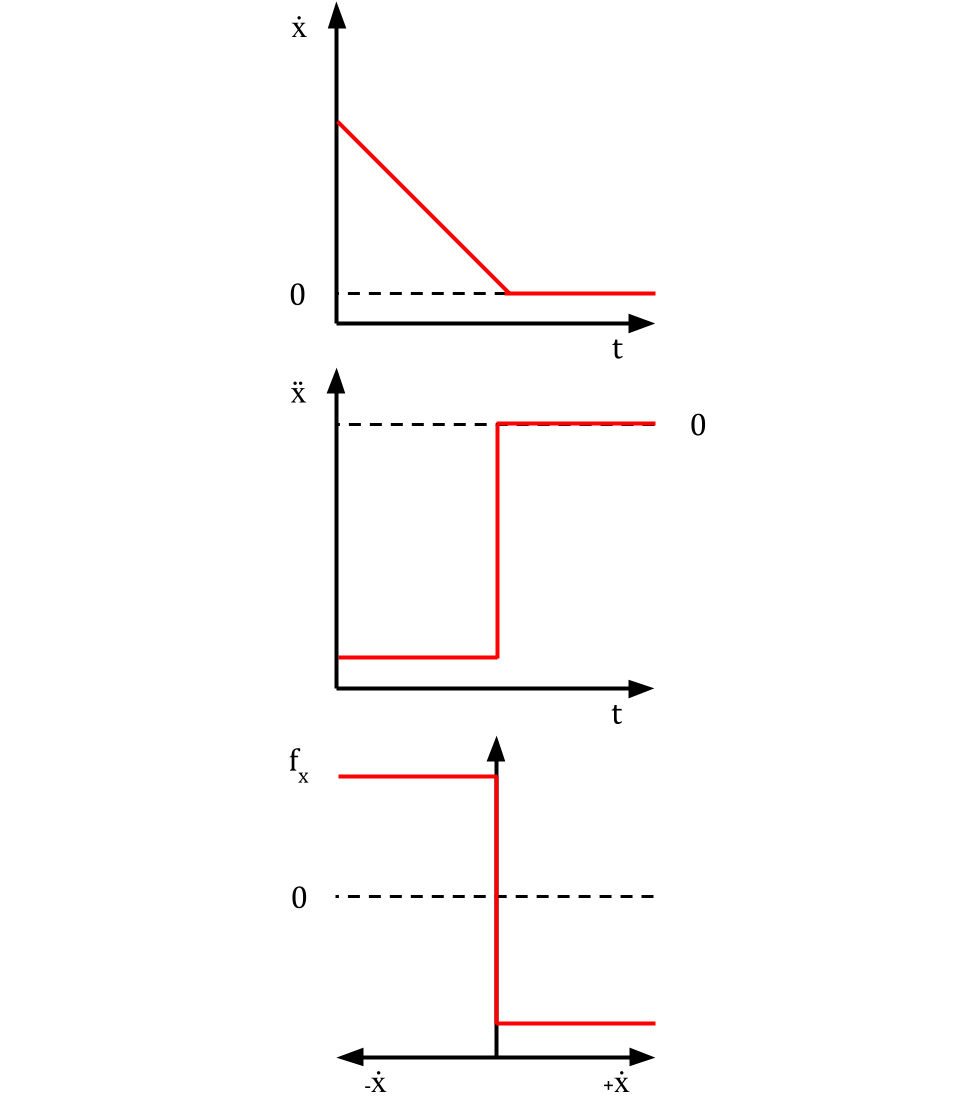
As your object transitions from slipping to sticking, your acceleration $\ddot{x}$ and friction force $f_x$ jump from constant values to zero. Budge the object in either direction and your friction force will shoot to a constant positive or negative value on a dime.

Because the relationship between friction and speed is tricky to model, we need to split this equation up a bit. Firstly, we define the magnitude of the friction force as follows.

$$ \begin{equation} ||f_x|| \leq \mu f_z \end{equation} $$

You may be wondering how the magnitude of friction can be less than $\mu f_z$ all of a sudden. Well think about what happens when the object stops. Its friction force can’t be proportional to the normal force anymore, or it would never stop moving! To enforce $f_x = 0$ when the object is stopped, we’re going to use a Lagrange multiplier, $\lambda_k$, which represents the magnitude of the tangential ground velocity at timestep $k$.

$$ \begin{equation} \lambda_k (\mu f_z - ||f_x||) = 0 \end{equation} $$

As you can see, we are constraining $f_x$ so that it can only be zero when the tangential velocity is zero.

The magnitude of tangential velocity $\lambda_k$ is defined as shown. Eq. (5) is pulling double duty because it also enforces that $f_x$ must point in the opposite direction of $\dot{x}_k$.

$$ \begin{equation} \dot{x}_k + \lambda_k \frac{f_x}{||f_x||} = 0 \end{equation} $$

$$ \begin{equation} \lambda_k \geq 0 \end{equation} $$

The Optimization Problem

Just like last time, there are a few hacks we have to use to make the optimization problem run well with IPOPT. Firstly, we have to define a “smooth square root” function, $\text{ssqrt}(x)$, as shown, to make norm functions less discontinuous. $\epsilon$ is an arbitrarily small constant that we will make equal to the solver tolerance.

$$ \begin{equation} \text{ssqrt}(x) = \sqrt{x + \epsilon^2} - \epsilon \end{equation} $$

$$ \begin{equation} || f_x || \approx \text{ssqrt}(f_x^2) \end{equation} $$

The optimization problem is as follows.

An explanation of what’s going on here:

• Eqs. (10) through (14) are the contact constraints we covered in the last post. The original slack variable is now denoted as $s_1$.
• Eq. (15) is Eq. (5), but smoothed, plus an additional $\epsilon$ to prevent division by zero.
• Eq. (16) is Eq. (3) smoothed.
• Eq. (17) is Eq. (4) with a second slack variable, $s_2$.

Note that I am using $f_x$ and $f_z$ to refer to the elements of the force vector at timestep $k$ to avoid complicating the notation.

Furthermore, assume that any slack variables mentioned ($s_1$ and $s_2$) are also taken at timestep $k$.

Now that that’s out of the way, let’s look at the code.

The Code

We start out by defining the “smooth square root” function, the solver tolerance, the 2D dynamics, and the integrator.

import numpy as np
import casadi as cs

import plotting

ϵ = 1e-4


def smoothsqrt(x):
    return cs.sqrt(x + ϵ * ϵ) - ϵ


n_a = 4  # length of state vector
n_u = 2  # length of control vector

m = 10  # mass of the particle in kg
g = 9.81  # gravitational constant
A = np.array([[0, 0, 1, 0], [0, 0, 0, 1], [0, 0, 0, 0], [0, 0, 0, 0]])
B = np.array([[0, 0], [0, 0], [1 / m, 0], [0, 1 / m]])
G = np.array([[0, 0, 0, -g]]).T
dt = 0.001  # timestep size
mu = 0.1  # coefficient of friction


def dynamics_ct(X, U):
    dX = A @ X + B @ U + G.flatten()
    return dX


def integrator_euler_semi_implicit(dyn_ct, xk, uk, xk1):
    xk_semi = cs.SX.zeros(n_a)
    xk_semi[:2] = xk[:2]
    xk_semi[2:] = xk1[2:]
    X_next = xk + dt * dyn_ct(xk_semi, uk)
    return X_next

Next, we set up the solver.

N = 1200  # number of timesteps
X_hist = np.zeros((N, n_a))  # array of state vectors for each timestep
Fx_hist = np.zeros(N)  # array of x friction forces for each timestep
Fz_hist = np.zeros(N)  # array of z GRF forces for each timestep
X_hist[0, :] = np.array([[0, 1, 1, 0]])
U_hist = np.zeros((N - 1, n_u))  # array of control vectors for each timestep

# initialize casadi variables
Xk1 = cs.SX.sym("Xk1", n_a)  # X(k+1), state at next timestep
F = cs.SX.sym("F", n_u)  # forces
s1 = cs.SX.sym("s1", 1)  # slack variable 1
s2 = cs.SX.sym("s2", 1)  # slack variable 2
lam = cs.SX.sym("lam", 1)  # lagrange mult for ground vel
X = cs.SX.sym("X", n_a)  # state
U = cs.SX.sym("U", n_u)  # controls

xk = X[0]
zk = X[1]
dxk = X[2]
Fx = F[0]  # friction force
Fz = F[1]  # grf

xk1 = Xk1[0]  # horz pos
zk1 = Xk1[1]  # vert pos

# objective function
obj = s1**2 + s2**2

constr = []  # init constraints
# dynamics
constr = cs.vertcat(
    constr, cs.SX(integrator_euler_semi_implicit(dynamics_ct, X, U + F, Xk1) - Xk1)
)

# tang. gnd vel is zero if GRF is zero but is otherwise equal to dx
# max dissipation
constr = cs.vertcat(constr, cs.SX(dxk + lam * Fx / (smoothsqrt(Fx * Fx) + ϵ)))

# primal feasibility
primal_friction = mu * Fz - smoothsqrt(Fx * Fx)  # uN = Ff
constr = cs.vertcat(constr, cs.SX(primal_friction))  # friction cone

# relaxed complementarity aka compl. slackness
constr = cs.vertcat(constr, cs.SX(s1 - Fz * zk1))  # ground penetration
constr = cs.vertcat(constr, cs.SX(s2 - lam * primal_friction))  # friction

opt_variables = cs.vertcat(Xk1, F, s1, s2, lam)
parameters = cs.vertcat(X, U)
lcp = {"x": opt_variables, "p": parameters, "f": obj, "g": constr}
opts = {
    "print_time": 0,
    "ipopt.print_level": 0,
    "ipopt.tol": ϵ,
    "ipopt.max_iter": 2000,
}
solver = cs.nlpsol("S", "ipopt", lcp, opts)

Then we define our constraint bounds.

n_var = np.shape(opt_variables)[0]
n_par = np.shape(parameters)[0]
n_g = np.shape(constr)[0]

# variable bounds
ubx = [1e10] * n_var
lbx = [0] * n_var  # dual feasibility
lbx[0] = -1e10  # set x unlimited
lbx[2] = -1e10  # set dx unlimited
lbx[3] = -1e10  # set dz unlimited
lbx[n_a] = -1e10  # set Fx unlimited

# constraint bounds
ubg = [1e10] * n_g
ubg[0:n_a] = np.zeros(n_a)  # set dynamics = 0
ubg[n_a] = 0  # set max dissipation = 0
lbg = [0] * n_g

Finally, we step through the simulation.

# run the sim
p_values = np.zeros(n_par)
x0_values = np.zeros(n_var)
s1_hist = np.zeros(N)
s2_hist = np.zeros(N)
lam_hist = np.zeros(N)
for k in range(N - 1):
    print("timestep = ", k)
    p_values[:n_a] = X_hist[k, :]
    p_values[n_a:] = U_hist[k, :]
    x0_values[:n_a] = X_hist[k, :]
    sol = solver(lbx=lbx, ubx=ubx, lbg=lbg, ubg=ubg, p=p_values, x0=x0_values)
    X_hist[k + 1, :] = np.reshape(sol["x"][0:n_a], (-1,))
    Fx_hist[k] = sol["x"][n_a]
    Fz_hist[k] = sol["x"][n_a + 1]
    s1_hist[k] = sol["x"][n_a + 2]
    s2_hist[k] = sol["x"][n_a + 3]
    lam_hist[k] = sol["x"][n_a + 4]

x_hist = X_hist[:, 0]
z_hist = X_hist[:, 1]
dx_hist = X_hist[:, 2]
dz_hist = X_hist[:, 3]

Click here for the full code.

Here’s the result.

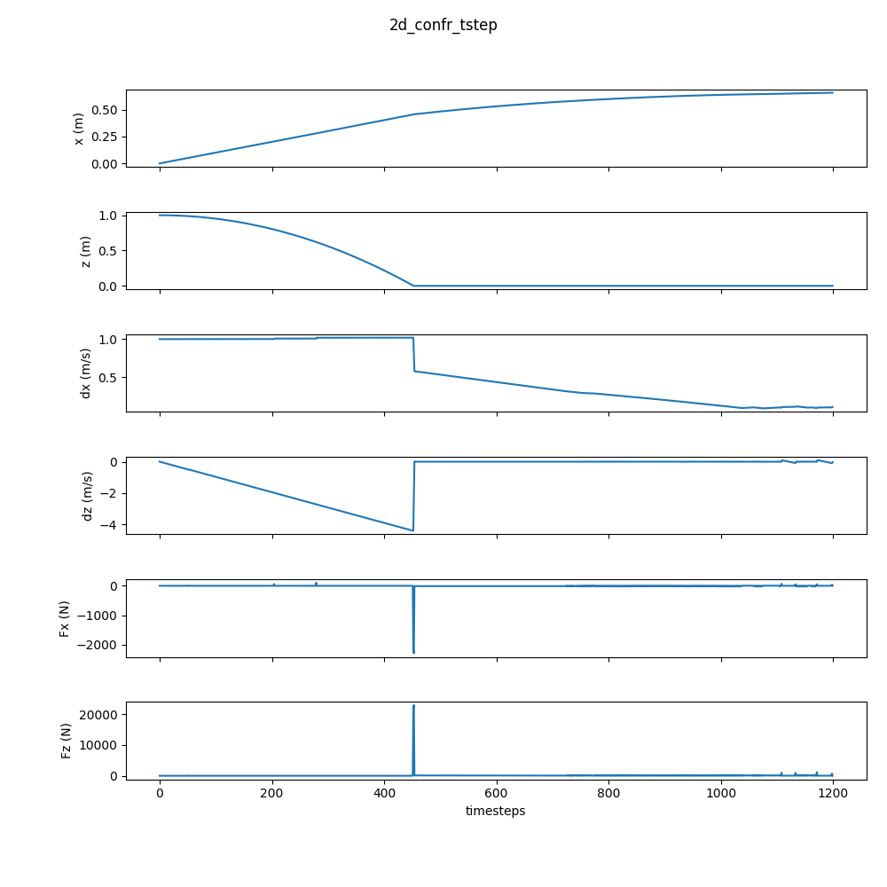
Neat! Although the plot looks a little messy–again, IPOPT is not really the right solver for this.

A Note on Friction with Hybrid and Smooth Contact

With the smooth and hybrid contact models, friction is simple enough that I’m not going to cover them here. I’m just going to provide example code below.

2D Hybrid Contact + Friction

2D Smooth Contact + Friction

Appendix

If you want to learn more about this stuff, check out these sources.

16-715: Simulating Coulomb Friction

SIGGRAPH'22 Course: Contact and Friction Simulation for Computer Graphics